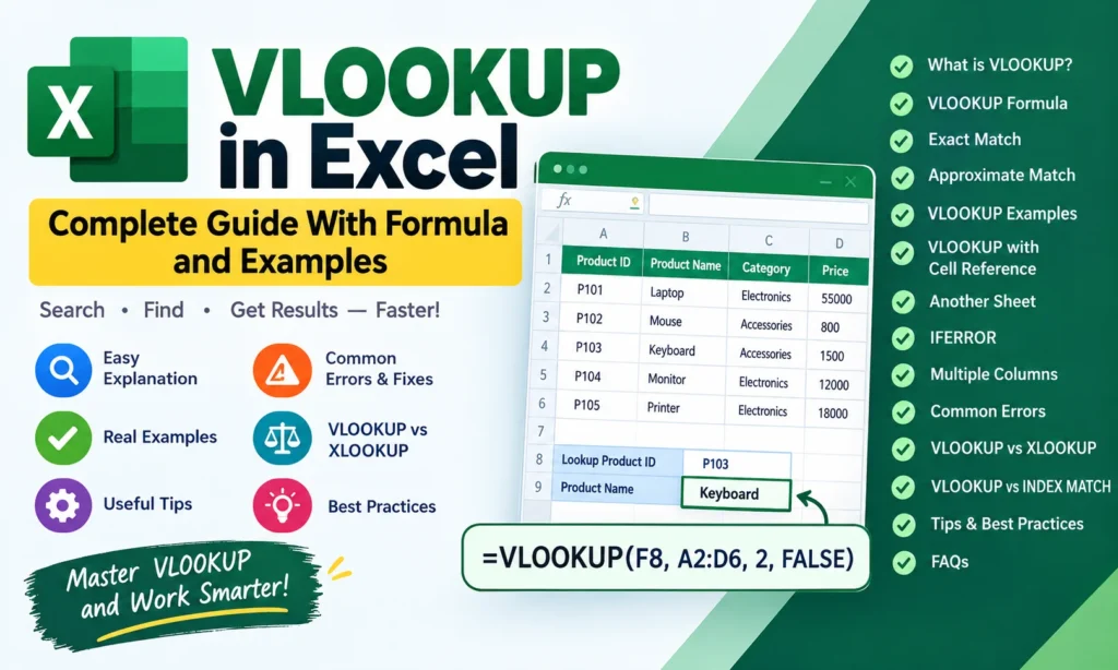
In this guide
- What Is VLOOKUP in Excel?
- Why Is VLOOKUP Important?
- VLOOKUP Syntax
- 1. lookup_value
- 2. table_array
- 3. col_index_num
- 4. range_lookup
- Finding an Employee’s Department
- Finding an Employee’s Salary
- Exact Match
- Approximate Match
- 1. #N/A Error
- 2. #REF! Error
- 3. #VALUE! Error
- 4. Wrong Result
- 1. Inventory Management
- 2. Employee Management
- 3. Sales Reports
- 4. Invoice Creation
- 5. Student Records
- 6. Customer Databases
- Use FALSE for Exact Matching
- Lock Your Table Range
- Keep the Lookup Column First
- Keep Data Clean
- Use IFERROR
- Use Named Ranges
- What does VLOOKUP mean in Excel?
- What is the basic VLOOKUP formula?
- Should I use TRUE or FALSE in VLOOKUP?
- Why is VLOOKUP returning #N/A?
- Can VLOOKUP search from right to left?
- Can VLOOKUP work between worksheets?
- Can VLOOKUP work between different workbooks?
- What is better than VLOOKUP?
- Can VLOOKUP return multiple results?
- How do I hide VLOOKUP errors?
VLOOKUP is one of the most useful and widely used functions in Microsoft Excel. Whether you are a student, accountant, business owner, data analyst, office professional, or someone who regularly works with spreadsheets, learning VLOOKUP can save you a significant amount of time.
When working with large Excel worksheets, you often need to find specific information from a table. For example, you may have a product ID and want to find its product name, price, category, or stock quantity. Instead of manually searching through hundreds or thousands of rows, you can use the VLOOKUP function in Excel to find the required information automatically.
In this comprehensive guide, we will explain what VLOOKUP is, how it works, its syntax, how to use it with practical examples, common errors, exact and approximate matching, limitations, and useful alternatives such as XLOOKUP and INDEX-MATCH.
What Is VLOOKUP in Excel?
VLOOKUP stands for Vertical Lookup. It is an Excel function used to search for a value in the first column of a table and return a related value from another column in the same row.
The function is called VLOOKUP because it searches vertically down the first column of a selected table.
For example, imagine you have this table:
| Product ID | Product Name | Category | Price |
|---|---|---|---|
| P101 | Laptop | Electronics | 55000 |
| P102 | Keyboard | Accessories | 1200 |
| P103 | Mouse | Accessories | 700 |
| P104 | Monitor | Electronics | 15000 |
If you enter the Product ID P103 and want Excel to automatically return the product name, you can use VLOOKUP.
The formula would be:
=VLOOKUP("P103",A2:D5,2,FALSE)
Excel searches for P103 in the first column of the table and returns the value from the second column, which is Mouse.
Why Is VLOOKUP Important?
VLOOKUP is particularly useful when you work with large amounts of structured data.
Some common applications include:
- Finding employee information
- Searching product prices
- Matching customer IDs
- Retrieving student marks
- Finding sales information
- Creating invoices
- Managing inventory
- Comparing databases
- Generating reports
- Combining information from different tables
- Automating repetitive spreadsheet tasks
Instead of manually searching for information, you can create a formula that retrieves it automatically.
VLOOKUP Syntax
The basic syntax of VLOOKUP is:
=VLOOKUP(lookup_value, table_array, col_index_num, [range_lookup])
Let’s understand each argument.
1. lookup_value
The lookup_value is the value you want Excel to find.
For example:
=P101
or:
"John"
It can be a number, text, cell reference, or another formula result.
2. table_array
The table_array is the range containing the data you want Excel to search.
For example:
A2:D100
The most important rule is that the lookup value must be located in the first column of the table_array.
3. col_index_num
This tells Excel which column’s value should be returned.
For example, if your table contains four columns:
| Column | Information |
|---|---|
| 1 | Product ID |
| 2 | Product Name |
| 3 | Category |
| 4 | Price |
Then:
2
returns the Product Name.
And:
4
returns the Price.
4. range_lookup
This determines whether you want an exact or approximate match.
There are two main options:
FALSE
for an exact match.
And:
TRUE
for an approximate match.
For most everyday lookup tasks, FALSE is usually the safer choice.
How to Use VLOOKUP in Excel
Let’s use a practical example.
Suppose you have the following employee table:
| Employee ID | Name | Department | Salary |
|---|---|---|---|
| E101 | Rahul | Sales | 35000 |
| E102 | Priya | HR | 40000 |
| E103 | Amit | IT | 55000 |
| E104 | Neha | Marketing | 45000 |
Suppose cell F2 contains:
E103
You want Excel to return the employee’s name.
Use:
=VLOOKUP(F2,A2:D5,2,FALSE)
The formula searches for the value in F2 in the first column of A2:D5.
Because the Name column is the second column, we use:
2
The result will be:
Amit
Finding an Employee’s Department
To retrieve the department, use:
=VLOOKUP(F2,A2:D5,3,FALSE)
The result will be:
IT
Finding an Employee’s Salary
To retrieve the salary:
=VLOOKUP(F2,A2:D5,4,FALSE)
The result will be:
55000
This demonstrates how changing the column index changes the returned information.
Exact Match vs Approximate Match in VLOOKUP
Understanding the difference between exact and approximate matching is extremely important.
Exact Match
For an exact match, use:
FALSE
or:
0
Example:
=VLOOKUP(A2,D2:G100,3,FALSE)
Excel will look for the exact value.
If it cannot find the value, it generally returns:
#N/A
Exact matching is ideal for:
- Employee IDs
- Product IDs
- Invoice numbers
- Customer IDs
- Roll numbers
- Account numbers
- Serial numbers
Approximate Match
For approximate matching, use:
TRUE
or:
1
Example:
=VLOOKUP(A2,D2:E10,2,TRUE)
Approximate matching is useful for ranges such as:
- Tax brackets
- Commission rates
- Grade systems
- Discount levels
- Pricing tiers
- Shipping rates
The first column of the lookup table should generally be sorted in ascending order when using approximate matching.
VLOOKUP With Cell References
Instead of typing the lookup value directly into the formula, it is better to use a cell reference.
Suppose:
A2 = P103
and your data is in:
D2:G100
You could use:
=VLOOKUP(A2,D2:G100,2,FALSE)
Now, if A2 changes from P103 to P104, the result automatically changes.
This makes VLOOKUP especially useful for interactive spreadsheets.
VLOOKUP With Absolute Cell References
When copying a VLOOKUP formula down multiple rows, it is often important to lock the table range.
For example:
=VLOOKUP(A2,$D$2:$G$100,2,FALSE)
The dollar signs make the range absolute.
Without absolute references, Excel may change the range when you copy the formula.
For example, a formula copied down could unintentionally change:
D2:G100
to:
D3:G101
Using:
$D$2:$G$100
keeps the lookup range fixed.
Using VLOOKUP Across Different Worksheets
VLOOKUP can also retrieve information from another worksheet.
Suppose your lookup value is on Sheet1 and your data is stored on Sheet2.
You can use:
=VLOOKUP(A2,Sheet2!A:D,2,FALSE)
This tells Excel to search for A2 in columns A through D of Sheet2.
For example, if Sheet2 contains product information and Sheet1 contains an order form, VLOOKUP can automatically bring the product name and price into the order form.
This is one of the most practical uses of VLOOKUP in business spreadsheets.
VLOOKUP Between Different Excel Workbooks
You can also use VLOOKUP to retrieve information from another Excel workbook.
For example:
=VLOOKUP(A2,'[Products.xlsx]Sheet1'!$A$2:$D$500,4,FALSE)
The exact reference will depend on the workbook and worksheet names.
This can be useful when maintaining separate files for:
- Inventory
- Customers
- Employees
- Sales
- Products
- Accounting
However, external workbook links should be managed carefully because moving or renaming the source workbook can cause broken references.
VLOOKUP With Text Values
VLOOKUP works with text as well as numbers.
Suppose your table contains:
| Code | Product |
|---|---|
| A101 | Laptop |
| A102 | Tablet |
| A103 | Printer |
You can use:
=VLOOKUP("A102",A2:B4,2,FALSE)
The result is:
Tablet
If your lookup value is in cell D2:
=VLOOKUP(D2,A2:B4,2,FALSE)
VLOOKUP With Numbers
VLOOKUP also works with numerical values.
For example:
| ID | Score |
|---|---|
| 101 | 85 |
| 102 | 90 |
| 103 | 78 |
Formula:
=VLOOKUP(102,A2:B4,2,FALSE)
Result:
90
Be careful when numbers are stored as text. A number such as 102 and text "102" may not behave as expected in certain lookup situations.
How to Handle VLOOKUP Errors
One of the most common problems with VLOOKUP is the #N/A error.
For example:
=VLOOKUP(A2,D2:E100,2,FALSE)
If Excel cannot find the value, it may return:
#N/A
You can make the result more user-friendly with IFERROR.
Use:
=IFERROR(VLOOKUP(A2,D2:E100,2,FALSE),"Not Found")
Instead of displaying an error, Excel will display:
Not Found
You can also use:
=IFERROR(VLOOKUP(A2,D2:E100,2,FALSE),"")
This displays a blank cell if the lookup fails.
Common VLOOKUP Errors
1. #N/A Error
This usually means Excel cannot find the lookup value.
Possible causes include:
- Incorrect lookup value
- Extra spaces
- Different data types
- Wrong lookup range
- Missing record
- Typing mistakes
Check that the lookup value actually exists in the first column.
2. #REF! Error
This can occur when the column index is greater than the number of columns in the selected table.
For example:
=VLOOKUP(A2,A2:D10,5,FALSE)
The table only contains four columns, but the formula requests column 5.
The correct index must be between 1 and 4.
3. #VALUE! Error
This can occur when one or more arguments in the formula are invalid.
Check the formula structure and make sure the column index is a valid number.
4. Wrong Result
Incorrect results often happen when:
- TRUE is used instead of FALSE
- The approximate lookup table is not sorted
- The wrong column index is selected
- Data contains inconsistent formatting
VLOOKUP and Duplicate Values
An important limitation of VLOOKUP is that it generally returns the first matching result it finds.
For example:
| Employee | Department |
|---|---|
| Amit | Sales |
| Amit | IT |
| Rahul | HR |
If you use:
=VLOOKUP("Amit",A2:B4,2,FALSE)
VLOOKUP will return:
Sales
It does not automatically return all matching Amit records.
If your dataset contains duplicates and you need multiple results, modern Excel functions such as FILTER may be more appropriate.
VLOOKUP From Left to Right
Traditional VLOOKUP searches the first column and returns a value from a column to the right.
For example:
| ID | Name | Salary |
|---|---|---|
| 101 | Amit | 50000 |
| 102 | Rahul | 60000 |
You can search for ID and return Name or Salary.
But VLOOKUP cannot directly search a column to the right and return a value from a column to the left.
This is one of its major limitations.
VLOOKUP vs XLOOKUP
Modern versions of Excel include XLOOKUP, which is more flexible than VLOOKUP in many situations.
A VLOOKUP formula might look like:
=VLOOKUP(A2,D2:G100,4,FALSE)
An XLOOKUP equivalent could be:
=XLOOKUP(A2,D2:D100,G2:G100,"Not Found")
XLOOKUP can:
- Search left or right
- Return custom messages
- Avoid column-number counting
- Perform exact matching more conveniently
- Work with separate lookup and return ranges
If your Excel version supports XLOOKUP, it is often worth learning.
However, VLOOKUP remains extremely important because it is widely used in existing spreadsheets, business templates, tutorials, and older Excel versions.
VLOOKUP vs INDEX-MATCH
Another powerful alternative is the combination of INDEX and MATCH.
A traditional formula might be:
=INDEX(C2:C100,MATCH(A2,A2:A100,0))
INDEX-MATCH is more flexible than traditional VLOOKUP and can search in either direction.
It is especially useful when:
- Column positions may change
- You need left-side lookups
- You work with complex spreadsheets
- You want more control over lookup logic
Still, VLOOKUP is generally easier for beginners to understand.
Practical Business Uses of VLOOKUP
1. Inventory Management
Businesses can maintain a product database and automatically retrieve prices, categories, suppliers, or stock levels using product IDs.
For example:
=VLOOKUP(A2,Products!A:E,5,FALSE)
This could return the available stock quantity.
2. Employee Management
HR teams can use VLOOKUP to retrieve employee departments, salaries, joining dates, or job titles.
3. Sales Reports
Sales teams can match customer IDs with customer names, regions, sales targets, or account managers.
4. Invoice Creation
A product code can automatically populate:
- Product name
- Price
- Tax category
- Product description
This reduces manual data entry.
5. Student Records
Schools and educational institutions can use VLOOKUP to retrieve:
- Student names
- Marks
- Classes
- Grades
- Subjects
6. Customer Databases
Customer IDs can be used to retrieve contact information, account details, order information, or customer categories.
Tips for Using VLOOKUP Effectively
Use FALSE for Exact Matching
For IDs and unique records, prefer:
FALSE
unless you specifically need approximate matching.
Lock Your Table Range
Use absolute references:
$A$2:$D$500
when copying formulas.
Keep the Lookup Column First
Remember that traditional VLOOKUP searches only the first column of the selected table.
Keep Data Clean
Remove unnecessary spaces and make sure numbers and text are stored consistently.
Use IFERROR
For cleaner spreadsheets:
=IFERROR(VLOOKUP(A2,D:E,2,FALSE),"Not Found")
Use Named Ranges
For large workbooks, named ranges can make formulas easier to understand.
For example:
=VLOOKUP(A2,ProductTable,3,FALSE)
can be easier to maintain than a large cell reference.
VLOOKUP Best Practices
A good Excel workbook should be designed with consistency and maintainability in mind.
First, keep your source data organized in a proper table. Avoid unnecessary blank rows and columns.
Second, use clear column headings.
Third, make sure the lookup column contains unique values whenever possible.
Fourth, use exact matching when searching for unique IDs.
Fifth, use absolute references when copying formulas.
Finally, consider using XLOOKUP or other modern Excel functions if your version supports them and your requirements are more advanced.
VLOOKUP Example for a Product Price List
Consider the following table:
| Product Code | Product | Category | Price |
|---|---|---|---|
| P001 | Laptop | Electronics | 55000 |
| P002 | Smartphone | Electronics | 25000 |
| P003 | Keyboard | Accessories | 1500 |
| P004 | Mouse | Accessories | 800 |
| P005 | Monitor | Electronics | 12000 |
If cell F2 contains:
P004
To find the product name:
=VLOOKUP(F2,A2:D6,2,FALSE)
Result:
Mouse
To find the category:
=VLOOKUP(F2,A2:D6,3,FALSE)
Result:
Accessories
To find the price:
=VLOOKUP(F2,A2:D6,4,FALSE)
Result:
800
This simple example demonstrates how a single product code can be used to retrieve multiple pieces of information.
How to Make VLOOKUP Dynamic
You can make your spreadsheet interactive by allowing users to enter a lookup value into one cell.
For example:
Enter Product Code: P003
Then formulas can automatically retrieve the product details.
Product name:
=IFERROR(VLOOKUP(F2,A2:D100,2,FALSE),"Not Found")
Category:
=IFERROR(VLOOKUP(F2,A2:D100,3,FALSE),"Not Found")
Price:
=IFERROR(VLOOKUP(F2,A2:D100,4,FALSE),"Not Found")
This approach can be used to build simple search tools, dashboards, invoice systems, inventory sheets, and reporting templates.
VLOOKUP Limitations You Should Know
Although VLOOKUP is powerful, it is not perfect.
Some important limitations include:
- It normally searches only the first column of the selected table.
- It cannot directly return values from columns to the left.
- It can become difficult to maintain when column numbers change.
- Duplicate lookup values can produce unexpected results.
- Approximate matching requires properly sorted data.
- Large and complex VLOOKUP formulas can affect workbook performance.
- It may not be the best choice for multiple-result searches.
Understanding these limitations helps you choose the right Excel function for each situation.
Frequently Asked Questions About VLOOKUP
What does VLOOKUP mean in Excel?
VLOOKUP means Vertical Lookup. It searches for a value in the first column of a table and returns related information from another column in the same row.
What is the basic VLOOKUP formula?
The basic syntax is:
=VLOOKUP(lookup_value,table_array,col_index_num,range_lookup)
Should I use TRUE or FALSE in VLOOKUP?
For most exact lookup tasks, use:
FALSE
TRUE is mainly useful for approximate matching and range-based lookups.
Why is VLOOKUP returning #N/A?
Usually because Excel cannot find the lookup value. Check the lookup value, source data, spaces, formatting, and selected range.
Can VLOOKUP search from right to left?
Traditional VLOOKUP cannot directly return a value from a column to the left of the lookup column. XLOOKUP or INDEX-MATCH can handle this more flexibly.
Can VLOOKUP work between worksheets?
Yes. For example:
=VLOOKUP(A2,Sheet2!A:D,2,FALSE)
Can VLOOKUP work between different workbooks?
Yes. VLOOKUP can reference another Excel workbook, although external links should be managed carefully.
What is better than VLOOKUP?
For newer versions of Excel, XLOOKUP is often more flexible. INDEX-MATCH is another powerful alternative.
Can VLOOKUP return multiple results?
Traditional VLOOKUP generally returns only the first matching result. Functions such as FILTER can be better when multiple matching records are required.
How do I hide VLOOKUP errors?
Use IFERROR:
=IFERROR(VLOOKUP(A2,D2:E100,2,FALSE),"Not Found")
Conclusion
VLOOKUP remains one of the most valuable Excel functions for searching and retrieving information from structured data. Once you understand its four main arguments—lookup value, table array, column index number, and range lookup—you can use it for a wide variety of real-world spreadsheet tasks.
For basic employee databases, product lists, sales reports, inventory systems, invoices, student records, and customer databases, VLOOKUP can significantly reduce manual work and improve spreadsheet accuracy.
The most important habit to develop is knowing when to use an exact match. For unique IDs, product codes, customer numbers, and similar records, the following structure is often the most useful:
=VLOOKUP(A2,TableRange,ColumnNumber,FALSE)
You should also learn how to use absolute references, IFERROR, worksheet references, and clean source data. Once you are comfortable with these techniques, you can create much more powerful Excel worksheets.
Although newer functions such as XLOOKUP provide additional flexibility, VLOOKUP is still worth learning because it is widely supported and frequently appears in existing Excel files, business templates, workplace tasks, tutorials, and data-processing workflows.
If you regularly work with Excel, mastering VLOOKUP is an excellent step toward becoming more efficient and confident with spreadsheet data analysis.